Methodological Approach

To answer our research question, we need to be able to find the routes through Zurich that offer the most shade at a particular time of day, during a particular part of the year. Since the additional heat stress of Urban Heat Islands is particularly felt during hot summer days, we decided to investigate shaded routes during the months of June, July and August.

Data Preparation

In order to find the most shaded routes through Zurich, we first needed to find out which areas of Zurich would be shaded and to what extent during different times of day. It became apparent that we would need to calculate the cast shadows in the city ourselves, since official shadow maps of Zurich do not exist.

As a first step we looked for a Digital Surface Model (DSM) of Zurich. A DSM represents the surface of the earth and all the different kinds of objects on it, like infrastructure (residential and commercial buildings, bridges, train stations etc.) and vegetation cover (Trees, bushes etc.). We eventually found and downloaded the current DSM of the city of Zurich “Digitale Höhenmodelle aktuell ZH (2022)”. Since we concentrated on the inner city of Zurich, the DSM was clipped to our area of interest (AOI).

In the next step we imported the clipped DSM into ArcGIS, where we used the “Raster Solar Radiation” tool to create our shadows. Given a DSM as input, the tool calculates how much solar radiation a given area receives during a given timeframe. Using the clipped DSM, we calculated the incoming Solar Radiation for each pixel of the DSM for the 15th of June, July and August during 09:00, 12:00 and 15:00 o'clock.

Why did we choose these specific dates and times? Calculating the solar radiation for each pixel for every day of the three months would take up too much computer memory for it to be feasible to host on our own. Thus, we chose the 15th of every month as a kind of representative “middle ground” that would stand for the entire month. The specific times of day were chosen to show the differences in cast shadows between the morning, noon and afternoon.

We used the Solar Radiation values of the pixels as proxies for shadows, since low values (near 0) are synonymous with shadows, as they simply represent areas with low incoming light.

Since our interest was finding out which routes to travel on while avoiding as much sunlight as possible during specific times, we clipped our resulting Solar Radiation Rasters (SRS) to the street network of our AOI. Finding a polygonal street network data source with which we could achieve this proved challenging, since most available street network datasets were composed of lines. In the end we found the “AV MOpublic, Bodenbedeckung” dataset which contained roads and sidewalks in Zurich as polygons. Unfortunately, these street networks were not complete, often missing small parts and connections into dead ends between buildings. We therefore manually added the most crucial missing features, like parts of Hardbrücke and paths through the Hauptbahnhof, that were absent.

After clipping the SRS to the street network, we were left with nine rasters that represented solar radiation values on the streets of our AOI, during our chosen times. The last step in our data preparation was up-sampling the resolution of our raster files to a resolution of 4x4m for each raster pixel.

We also wanted users of our map to be able to observe when and where shadows were cast on the streets of our AOI. To achieve this, we converted our finalised SRS into web map tiles, which could later be toggled on and off as a map overlay. The same procedure was performed for an Urban Heat Island Layer, which showed how different parts of the AOI experienced differing amounts of additonal heat during the June, July and August.

Finding the most shaded paths

With our clipped and up-sampled SRS files we now faced the challenge of finding the most shaded path between any two points in our AOI. To achieve this, we employed the Least Cost Path (LCP) analysis, which estimates the path between a starting and end point on a surface with the least movement cost (Rees, 2004). In our case the cost surfaces were the clipped and up-sampled SRS, and the individual movement costs were the solar radiation values of the individual pixel. From the starting pixel, the LCP searches the surrounding eight pixels for the one with smallest value and moves to it– the least-cost movement. From this second pixel, the algorithm searches again for the neighbour with the least cost (excluding our starting point and all previous selected pixels). This process is repeated until the path that connects start and destination with smallest movement cost has been found.

Since we use solar radiation values and since the smaller radiation values mean less sunlight in a given pixel, this ultimately creates a route between two points on our SRS that has the least amount of sun exposure or, put another way, the most shaded path.

The LCP and as well as all the other parts of our web map were implemented in R and RShiny, and are hosted on shinyapps.io. To learn more about the design decision we made, visit the Design Principles tab.

Limitations

Our project is partial to a few technical limitations that might make themselves known during the use of our map.

As mentioned above, the street network we used to clip the SRS was not complete. This results in some holes in shaded areas with which we calculate the LCP. These holes can be observed in the map when toggling on the “Shaded Areas” map overlay. They mostly crop up where tram lines, roundabouts and other traffic features as well as trees are in the actual city. If the holes are selected as points, they theoretically can cause the LCP routing to fail because the values of their pixels count as “invalid” (NA). We implemented a fix that snaps invalidly selected points (those in buildings and raster holes) to the nearest valid raster pixel, so that these errors should not occur, but it remains a possibility in niche cases.

Another source of problems is the up-sampling of our SRS to 4x4m, from the original pixel size. This step was necessary, because our map is hosted on shinyapps.io, a web hosting service for apps built with the RShiny framework. Shinyapps.io offers a free tier of hosting services, which we use for our map. This free tier is limited in the file sizes and computing power that is available to our app. SRS with smaller, more accurate pixels lead to larger file sizes and require more computational power to calculate LCPs between two points. Through trial and error, we eventually found out, that a pixel size of 4x4m was the lowest pixel size we could use while still being able to use the free hosting tier. Larger pixel sizes led to crashing of the map, since the files were too large and the LCP computation took too much memory. These file size and memory limits are also why the shaded areas and the heat stress overlay can only be zoomed in on to a certain limit.

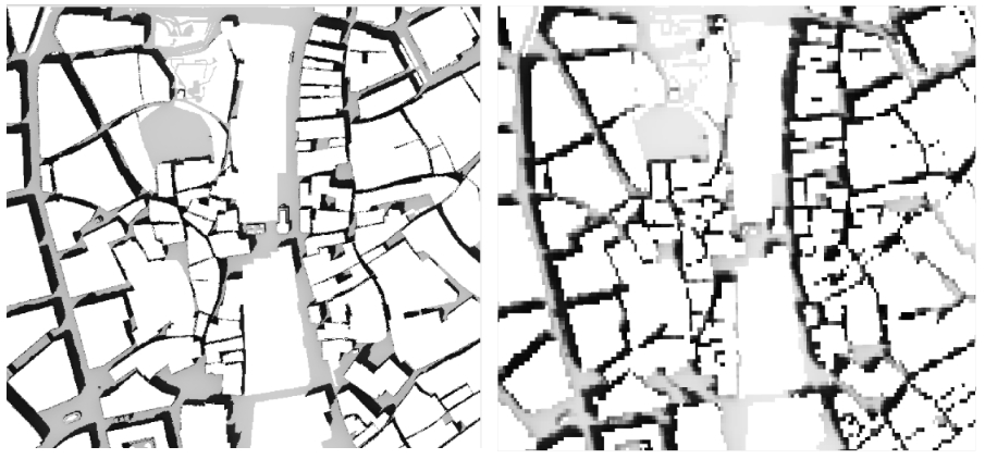
Larger pixel sizes lead to problems for the LCP. Through the up-sampling the connections between some areas of the map could not be maintained, as the pixel sizes grew so large that individual streets could sometimes only be represented through a few pixels that did not touch each other. This problem is especially apparent in the medieval city centre where very narrow streets are the norm. Navigating through them is often not possible or produces routes that take long or unnecessary detours. If such pixels are encountered during LCP calculation, the process is aborted and the error message “No connected path could be found” is displayed. The two pictures below illustrate this. The left image shows the SRS with its original pixel size, while the right image shows the up-sampled SRS. You may notice that the paths through the very small streets at the centre of the images are connected in the left image, while the coarser pixel size in the right image lead to some paths not being connected anymore.