Data

The analysis is carried out on a global scale for the time frame 1995 to 2020. Two main thematic data inputs were used to create this analysis: Greenhouse gas emissions and the GAIN-Index, both discussed in more detail here.

Greenhouse Gas Emissions

Greenhouse gas emissions are used to measure the contribution to climate change of each nation from 1995 to 2020. All used greenhouse gas data is from Climate Watch. The following greenhouse gases are considered:

• Carbon dioxide (CO2) emissions in tons per capita and year.
• Methane (CH4) emissions in tons of CO2-equivalent per capita and year.
• Nitrogen dioxide (NO2) emissions in tons of CO2-equivalent per capita and year.
• All greenhouse gases combined in tons of CO2-equivalent per capita and year.

For further information, please consult: Climate Watch.

Impact Index

To measure a nation's vulnerability and readiness to climate change from 1995 to 2020, an existing index is used called the GAIN index, calculated by Notre Dame Global Adaption Initiative. This index consists of a country's readiness and vulnerabily to climate change, thus describing its resiliance. A higher GAIN index score therefore indicates greater readiness and reduced vulnerability to climate change, making it advantageous for a nation. In this project however, a new index called impact index is used, which is simply calculated the following: 1 - GAIN index. This index can thereby be used to show how strongly a nation is potentially affected by climate change.

The impact index consists of a vulnerabiltiy and readiness index, which in turn are composed of more specific factors. These indices are normalized between 0 and 1, allowing for a comparison between them. All used data on the impact index is from University of Notre Dame.

Vulnerability Index

The vulnerability index is composed of the (adaptive) capacity, sensitivity and exposure of a nation. It considers the six life-supporting sectors: food, water, health, ecosystem services, human habitat, and infrastructure.

• Exposure: Refers to the extent to which a system faces substantial climate change impacts from a biophysical standpoint, omitting socio-economic factors.
• Sensitivity: Denotes the degree of reliance a country has on sectors that are adversely impacted by climate hazards, or the percentage of the population that is especially vulnerable to climate change hazards.
• Adaptive Capacity: Refers to the social resources accessible for sector-specific adaptation efforts.

The exact structure of the vulnerability index can be seen in the following table:

Readiness Index

This metric evaluates a country's capacity to utilize investments effectively and translate them into adaptation initiatives. The readiness index assesses the overall preparedness by examining three key components: economic readiness, governance readiness, and social readiness.

• Economic: Reflects a country's economic capacity to finalize investments aimed at implementing adaptation measures that mitigate vulnerability, thereby reducing sensitivity and enhancing adaptive capacity.
• Governance: Reflects institutional elements that facilitate the effective utilization of investment for adaptation purposes.
• Social: Encompasses various factors such as social equity, ICT infrastructure, education, and innovation that facilitate the flow of investment and foster adaptation initiatives.

The exact structure of the readiness index can be seen in the following table:

Calculation and Interpretation

The GAIN index is calculated accordingly:

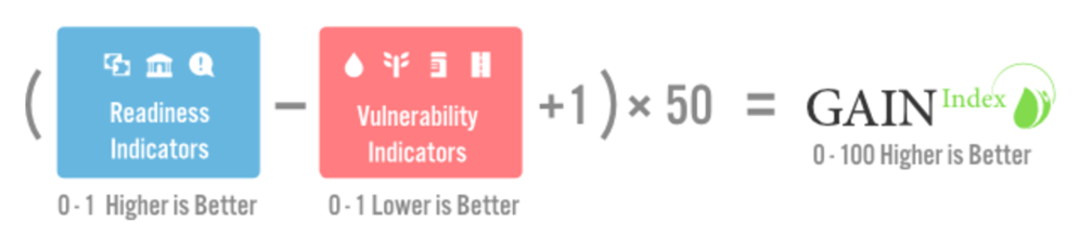
Therefore a higher GAIN index score indicates greater readiness and reduced vulnerability to climate change, making it advantageous for a nation:

Picture 3: University of Notre Dame 2024

The impact index is finally calculated with 1 - GAIN index.

For further information, please consult: Gain-Index.

Methods

All figures and maps were implemented with R Studio. For all datasets, countries were joined with their respective continents, allowing for statistical aggregation. Statistical aggregation to continent level is relevant for several interactive elements of the maps, such as the time series graph or the relationship analysis of impact and greenhouse gas emissions between continents. Continental and world averages of greenhouse gas emissions were weighted by the population of each nation before aggregation, allowing for accurate data comparison on higher aggregation levels. The Natural Breaks Jenks method was employed to determine class intervals for the maps. This method was chosen due to the dataset's characteristics, which include a wide range of emissions across nations. By employing the Natural Breaks Jenks method, the classification effectively groups nations with similar emission levels together, thus enhancing the visual contrast and facilitating a clearer understanding of the emission distribution. This was done by first logarithmising the data and then applying the natural jenks method. The datalimits were then transformed back to the original ones but with the classification of the logarithmised data. As a result, the outliers do not have such a strong influence and the distribution is more uniform. Finally, two maps side by side were chosen for the presentation of the data so that cause and impact can be compared directly between countries or regions of the world.

Target Audience

The maps are designed for a global audience, addressing the worldwide implications of climate change and the need for resilience to it. Given the universal relevance of this topic, it is crucial that the information is accessible to everyone. The maps should therefore be used and understood without prior cartographic knowledge, which is why we tried to make them simple and intuitive.

Limitations

During the implementation of the interactive map, there were some limitations that had to be overcome. Originally, the two maps should be linked so that when a year is selected, it is changed on both maps. However, this turned out to be quite difficult, as linking the data in R was rather complicated. Thus, in the end, we decided against linking both maps. This proved to be a good decision, as the maps run faster that way, as they run individually. Furthermore, one can also compare how past emissions influence the impact in the future, as emissions usually display a temporal offset between emission and impact. One issue that could not be resolved is the extended run-time of the maps. The issue occurs for two reasons. Firstly, the R server where the R shiny app with the maps and graphs is hosted has limited capacity. Secondly, the code is currently designed to recalculate the data for every change made in the interactive maps, as it references several synoptic datasets. To address this issue, we plan to implement individual files for each interactive element in the future. This will significantly reduce the need for real-time calculations. Additionally, the legend for the time series is interactive and follows a preset alphabetic order which causes the order of the legend to change between selected countries. This issue occurs because the graph and legend are interactive, meaning that the order of the legend cannot be predefined and made constant. Preferably, the order would be country, continent, world average. Our coding skills are not advanced enough to solve this issue.